open_dataset("data/person/") |>
  transmute(age_renamed = AGEP) |>
  show_query()
ExecPlan with 3 nodes:
2:SinkNode{}
1:ProjectNode{projection=["age_renamed": AGEP]}
0:SourceNode{}Bigger Data, Easier Workflows
In this chapter we’re going to dive into some more advanced topics. As we’ve shown in the previous chapters, the arrow R package includes support for hundreds of functions in R and has a rich type system. These empower you to solve most common data analysis problems. However, if you ever need to extend that set of functionality, there are several options.
To start, we’ll look in more detail at how bindings from R functions to Acero, the Arrow C++ query engine, work. We’ll also explore the converse of this: functions that exist in Acero and don’t have R equivalents, and how you can access these in your arrow pipelines. Then, we’re going to show how you can call back from Acero into R to do calculations where functions you want to use inside don’t have a corresponding Acero function. For other cases, we’ll show how the Arrow format’s focus on interoperability lets you stream data to and from other query engines, such as DuckDB, to access different functionality they have. Finally, we’ll look at a practical case of extending Arrow’s type system to work with geospatial data.
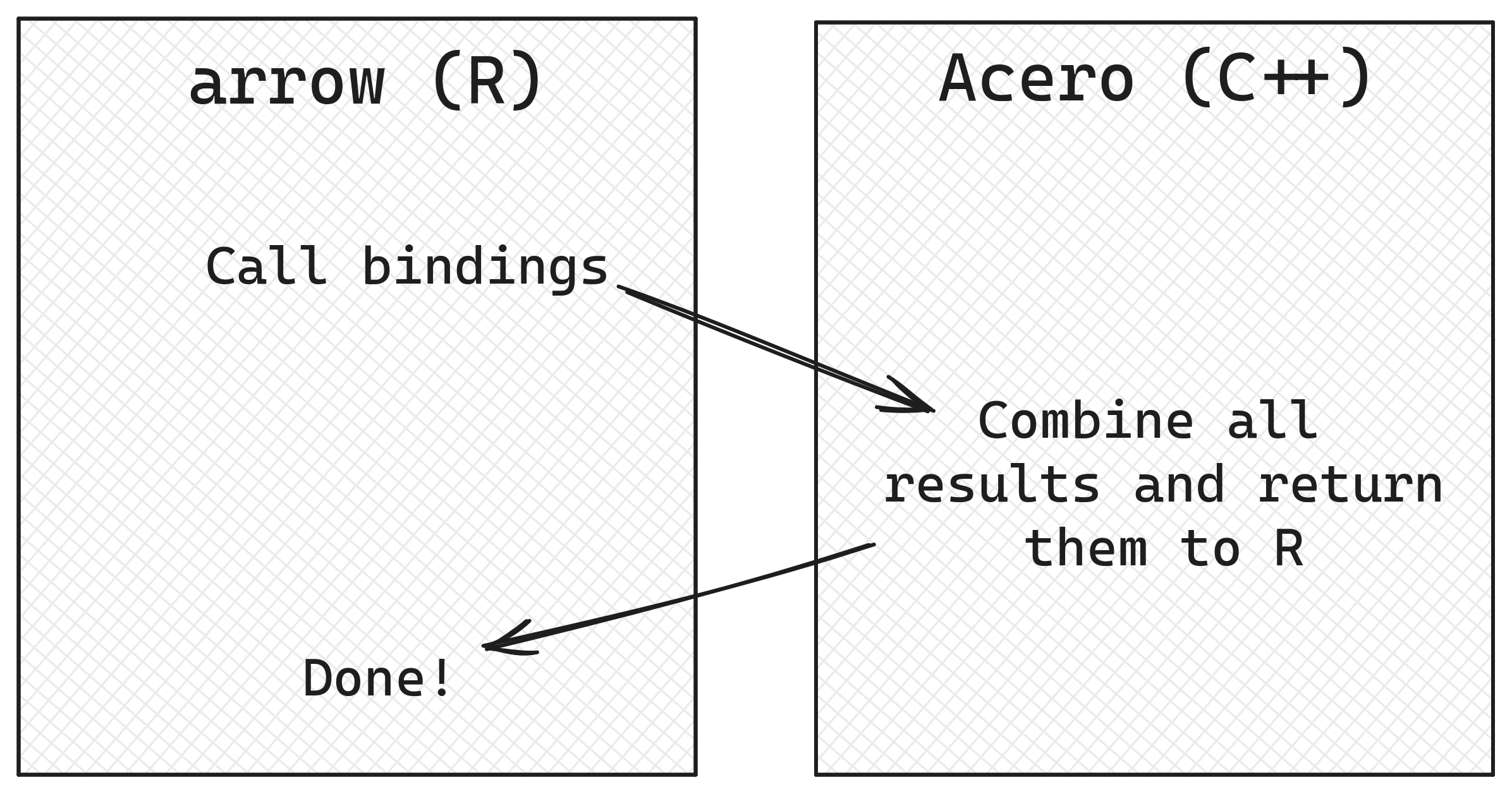
Acero is the Arrow C++ library’s query execution engine. A query execution engine is a library which allows users to perform queries against a data source. It takes input data and the operations to be performed on the data, combines them, and returns the output from this process.
It typically has multiple steps, which could include things like:
When you call dplyr functions on Arrow tabular objects like tables and datasets, the code in the R package translates this into execution plan—directed graphs that express what operations need to take place. These operations are represented by nodes. For example, a ProjectNode is used to create a new column.
You can see the execution plan by running show_query(), which displays the execution plan, as a final step in a query.
open_dataset("data/person/") |>
transmute(age_renamed = AGEP) |>
show_query()ExecPlan with 3 nodes:
2:SinkNode{}
1:ProjectNode{projection=["age_renamed": AGEP]}
0:SourceNode{}In the example above, the SourceNode and the SinkNode provide the input and the output. The middle step, the ProjectNode is where the new column is created.
A more complex query will end up with more nodes representing the different operations.
open_dataset("data/person/") |>
  filter(location == "wa") |>
  group_by(year) |>
  summarize(mean_age = mean(AGEP)) |>
  show_query()
ExecPlan with 5 nodes:
4:SinkNode{}
3:GroupByNode{keys=["year"], aggregates=[
hash_mean(mean_age, {skip_nulls=false, min_count=0}),
]}
2:ProjectNode{projection=["mean_age": AGEP, year]}
1:FilterNode{filter=(location == "wa")}
0:SourceNode{}Generally, we don’t have to worry about the details of these query plans, though they can be useful to get a closer look at exactly what is being run in Acero.
In Chapter 3, we mentioned that the arrow R package transforms dplyr syntax into Arrow Expressions which can be understood by Acero, and here we’re going to dive into that a little deeper.
Acero has a large number of functions implemented for performing calculations and transformations on data. The complete list can be found in the project documentation.
Some of these functions have the same names are the R equivalent. For example, both Acero and R have a min() function which can be used to find the lowest value in an vector or array of values. Other functions have slightly different names. While in R we use the - operator to subtract one value from another, in Acero, there are functions subtract() and subtract_checked(). The latter function is more commonly used as it accounts for overflow2 and raises an error if the value returned is beyond the minimum or maximum value for that data type.
Let’s take a closer look at an example.
The query below calculates a new column, the age of the respondents in the previous year, by deducting 1 from the value in the AGEP column. There is already a mapping between the - operator in R and subtract_checked() in Acero, and we can see this by creating our query but not actually executing it.
open_dataset("data/person/") |>
  transmute(age_previous_year = AGEP - 1)
FileSystemDataset (query)
age_previous_year: int32 (subtract_checked(AGEP, 1))
See $.data for the source Arrow objectWhen we print the query, the output shows that new column age_previous_year is calculated by calling the Acero function subtract_checked() and passing in a reference to the AGEP column and the number 1.
Mappings also exist for slightly more complex functions that have additional parameters.
Say we wanted to only return data for states whose names start with the letter “w”. We can take our dataset and use dplyr::filter() to return this subset, but we need to pick a function to pass to dplyr::filter() to actually do the filtering.
Let’s start first by looking at the Acero function we want Arrow to use. To be clear: we wouldn’t usually have to do this when working with arrow. This is just to illustrate how this all works.
If we look at the Acero compute function docs, we’ll see that there is a function starts_with which does this. It has 2 options: pattern, the substring to match at the start of the string, and ignore_case, whether the matching should be case sensitive.
So how do we use this from the arrow R package? We start off by considering which R function to use. Let’s go with the base R function startsWith(). Table 7.1 shows a comparison with the Acero equivalent.
sd with Acero’s stddev
| Function Name | Function Arguments | Prefix/Pattern Argument | Case Sensitivity | |
|---|---|---|---|---|
| R | startsWith |
prefix |
prefix: The prefix to match |
Always case-sensitive |
| Acero | starts_with |
pattern, ignore_case |
pattern: The pattern to match |
ignore_case: Boolean, set to false by default |
open_dataset("data/person/") |>
  select(location) |>
  filter(startsWith(x = location, prefix = "w"))
FileSystemDataset (query)
location: string
* Filter: starts_with(location, {pattern="w", ignore_case=false})
See $.data for the source Arrow objectThe information about the Acero mapping is shown here in the line which starts with “* Filter”. This contains a human-readable representation of the Arrow Expression created.
It shows that that startsWith() has been translated to the Acero function starts_with(). The options for the Acero function have been set based on the values which were passed in via the R expression. We set the startsWith() argument prefix to “w”, and that was passed to the Acero starts_with() option called pattern. As startsWith() is always case-sensitive, the Acero starts_with() option ignore_case has been set to false.
The arrow R package also has bindings for aggregation functions which take multiple rows of data and calculate a single values. For example, whereas R has sd() for calculating the standard deviation of a vector, Acero has stddev().
sd with Acero’s stddev
| Function Name | Function Options | Handling of Missing Values | Degrees of Freedom | Minimum Count | |
|---|---|---|---|---|---|
| R | sd |
na.rm |
na.rm: Boolean, removes NA values (default FALSE) |
Not implemented | Not implemented |
| Acero | stddev |
ddof, skip_nulls, min_count |
skip_nulls: Boolean, removes NULL values (default FALSE) |
ddof: Integer, denominator degrees of freedom (default 0) |
min_count: Integer, returns NULL if fewer non-null values are present (default 1) |
There are also some differences in the options for these functions; while R’s sd function has arguments x, the value to be passed in and na.rm, whether to remove NA values or not, Acero’s stddev also has ddof - denominator degrees of freedom, skip_nulls, the equivalent of na_rm, and min_count - if there are fewer values than this, return NULL.
open_dataset("data/person/") |>
  summarise(sd_age = sd(AGEP))
FileSystemDataset (query)
sd_age: double
See $.data for the source Arrow objectThe output here doesn’t show the function mapping as aggregation functions are handled differently from select(), filter(), and mutate(). The aggregation step is contained in the nested .data attribute of the query. This nesting ensures that the steps of the query are evaluated in this order. While select(), filter(), and mutate() can happen successively and be reflected in a single query step, any actions that happen on the data after summarize() (and, for that matter, joins) cannot be collapsed or rearranged like that.
You can see the full query by calling show_query() as a final step.
open_dataset("data/person/") |>
  summarise(sd_age = sd(AGEP)) |>
  show_query()
ExecPlan with 4 nodes:
3:SinkNode{}
2:ScalarAggregateNode{aggregates=[
stddev(sd_age, {ddof=1, skip_nulls=false, min_count=0}),
]}
1:ProjectNode{projection=["sd_age": AGEP]}
0:SourceNode{}We can see in the output above a references to the Acero stddev() function, as well as the values of the parameters passed to it.
We don’t have to know anything at all about about Acero functions in the typical case, where we know the R function we want to use, as arrow automatically translates it to the relevant Acero function if a binding does exist. But, what about if we want to use an Acero function which doesn’t have an R equivalent to start from?
We can view the full list of Acero functions available to use in arrow by calling list_compute_functions(). At the time of writing there were 262 Acero functions available to use in R - the first 20 are shown below.
list_compute_functions() |>
  head(20)
[1] "abs" "abs_checked" "acos"
[4] "acos_checked" "add" "add_checked"
[7] "all" "and" "and_kleene"
[10] "and_not" "and_not_kleene" "any"
[13] "approximate_median" "array_filter" "array_sort_indices"
[16] "array_take" "ascii_capitalize" "ascii_center"
[19] "ascii_is_alnum" "ascii_is_alpha" You can use these functions in your arrow dplyr pipelines by prefixing them with "arrow_".
This isn’t necessary when working with Acero functions which have a direct mapping to their R equivalents, which can be used instead. However, there are some niche use-cases where this could be helpful, such as if you want to use Acero options that don’t exist in the R equivalent function, or if there is no equivalent R function at all.
Let’s say that we wanted to do an analysis of the languages spoken by respondents in different areas. The columns we need for this analysis are:
LANP - the language spoken in each areaPWGTP - the weighting for that row in the datasetPUMA - a five digit number representing the smallest geographical area represented in the dataAlthough the PUMA code is number, as it can begin with a zero, it’s saved as a string. We know from having looked through the data that some rows in the dataset contain extra text, but for our analysis, we only want the rows in the dataset which contain only numbers in the PUMA column. We can use the Acero function utf8_is_digit(), which returns TRUE if a string contains only numbers and FALSE is there are any other characters in the string, to do this filtering.
open_dataset("data/person/") |>
  select(PUMA, LANP, PWGTP) |>
  filter(arrow_utf8_is_digit(PUMA))
FileSystemDataset (query)
PUMA: string
LANP: string
PWGTP: int32
* Filter: utf8_is_digit(PUMA)
See $.data for the source Arrow objectMost functions you want to use exist both in R and in Acero, and the arrow package has bindings that map the R syntax to the Acero functions. The previous section showed how to use Acero functions that don’t exist in R. But what if you want to use a R function which doesn’t have an Acero equivalent?
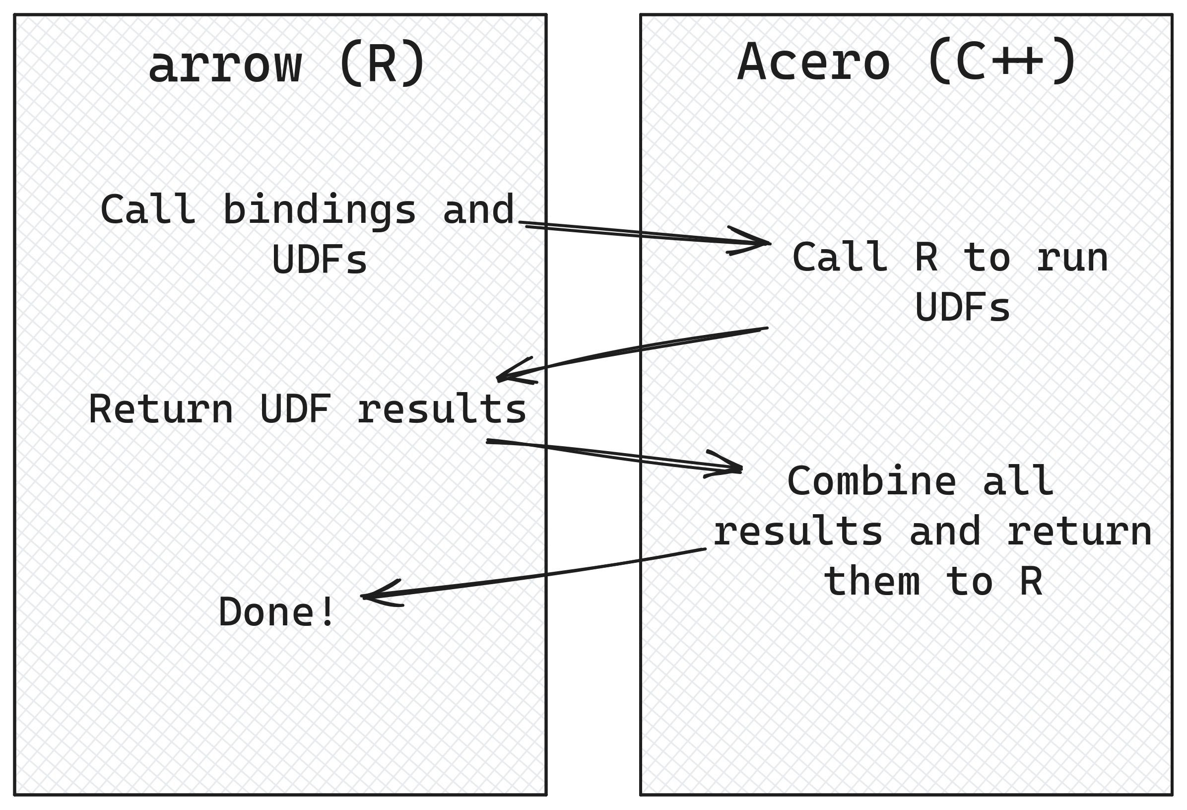
In this case, you can create a user-defined function (UDF). User-defined functions allow arrow to use functions that don’t have Acero bindings by calculating the results in your R session instead.
There is some additional processing overhead here because some of the calculation is being done by your R session and not by Acero, but it’s a helpful tool to have in these circumstances.
You can create a UDF by using the function register_scalar_function(). Let’s say we want to create a UDF which wraps the stringr function str_to_sentence(), which doesn’t have an Acero equivalent. Here’s an example of how it would look.
register_scalar_function(
  name = "str_to_sentence_udf",
  function(context, x) {
    stringr::str_to_sentence(x)
  },
  in_type = schema(
    x = string()
  ),
  out_type = string(),
  auto_convert = TRUE
)
Let’s walk through that one part at a time. The first thing we need to do is define the name we’d like to use to call the function later—in this case, str_to_sentence_udf. Next, define the function itself. The first argument must always be context—this is used by the C++ code to store metadata to help it convert data between R and C++, but you don’t need to do anything here manually other than name it as the first argument to your function. Next, define an argument which will be the columns in your dataset to use in the calculation, and any other values you need. In our case, we want the column representing the original string, which we’ve called x.
The body of the function itself is identical to when we defined it as an R function. The parameters in_type and out_type control the arrow data types of the input and output columns. Here, we provide a schema to in_type so that we can map function argument names to types, and we give a data type to out_type.
The auto_convert argument controls whether arrow automatically converts the inputs to R vectors or not. The default value, FALSE, means that inputs to your R function will be Arrow objects. In our example, this would mean that x would come in as an Arrow Array of type string(). But we want an R vector for x so that we can pass it to the stringr function. We could call as.vector() on x to convert the Array into an R vector, or we can do what we’ve done in this example and set auto_convert = TRUE to handle that for us. Setting auto_convert = TRUE also handles the return value conversion back to Arrow data for us.
Let’s take a look at how this UDF works with our data.
pums_person |>
  select(SOCP) |>
  mutate(SOCP = str_to_sentence_udf(SOCP)) |>
  head() |>
collect()Another example where UDFs can be useful is where you’ve created a model based on a subset of your data and you want to use it to make predictions. Let’s say we’ve created a linear model, using education and employment status to predict hours worked per week for respondents in 2018. When creating this model we aren’t using the standard stats::lm() because our data is weighted. The survey package has an equivalent regression function survey::svyglm() which applies the weights in the weight column during the regression. This isn’t strictly necesary for the demonstration here, but it does show how UDFs work not just with base R functions or functions in the tidyverse, but any R code that you come up with.
model_data <- open_dataset("data/person/") |>
    filter(year == 2018) |>
    filter(AGEP >= 16, AGEP < 65, !is.na(COW)) |>
    transmute(
      self_employed = str_detect(as.character(COW), "Self-employed"),
      edu = case_when(
        grepl("bachelor|associate|professional|doctorate|master", SCHL, TRUE) ~
          "College or higher",
        grepl("college", SCHL, TRUE) ~
          "Some college",
        grepl("High school graduate|high school diploma|GED", SCHL, TRUE) ~
          "High school",
        TRUE ~ "Less than High school"
      ),
      hours_worked = WKHP,
      PWGTP = PWGTP
    ) |>
    collect()

hours_worked_model <- survey::svyglm(
  hours_worked ~ self_employed * edu,
  design = survey::svydesign(ids = ~1, weights = ~PWGTP, data = model_data)
)
summary(hours_worked_model)
Call:
svyglm(formula = hours_worked ~ self_employed * edu, design = survey::svydesign(ids = ~1,
weights = ~PWGTP, data = model_data))
Survey design:
survey::svydesign(ids = ~1, weights = ~PWGTP, data = model_data)
Coefficients:
Estimate Std. Error t value Pr(>|t|)
(Intercept) 40.87539 0.01705 2397.62 <2e-16
self_employedTRUE -1.63441 0.08327 -19.63 <2e-16
eduHigh school -2.35634 0.03073 -76.67 <2e-16
eduLess than High school -6.66604 0.05241 -127.19 <2e-16
eduSome college -3.52614 0.03320 -106.22 <2e-16
self_employedTRUE:eduHigh school 2.61369 0.14297 18.28 <2e-16
self_employedTRUE:eduLess than High school 3.72725 0.19556 19.06 <2e-16
self_employedTRUE:eduSome college 2.77875 0.15217 18.26 <2e-16
(Intercept) ***
self_employedTRUE ***
eduHigh school ***
eduLess than High school ***
eduSome college ***
self_employedTRUE:eduHigh school ***
self_employedTRUE:eduLess than High school ***
self_employedTRUE:eduSome college ***
---
Signif. codes: 0 '***' 0.001 '**' 0.01 '*' 0.05 '.' 0.1 ' ' 1
(Dispersion parameter for gaussian family taken to be 152.4535)
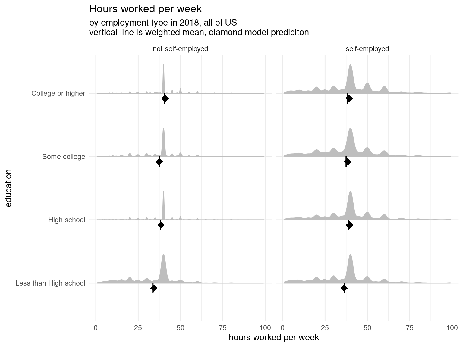
Number of Fisher Scoring iterations: 2We can use this model to predict what our model would have predicted on this data if it were new data coming in. This is a little artificial since this is the same data that we used to build the model, though it’s a good check to confirm that the modeling process doesn’t have anything terribly off about it. Also because we are predicting on the same data we fit this linear model on, this is going to be very close to the actual weighted means. We use the predict function to make these predictions and we also calculate the weighted mean for each group.
model_data$predicted <- predict(hours_worked_model, newdata = model_data)

model_data_summary <- model_data |>
  group_by(edu, self_employed) |>
  summarise(
    work_hours_mean = weighted.mean(hours_worked, w = PWGTP, na.rm = TRUE),
    work_hours_predicted = weighted.mean(predicted, w = PWGTP),
  )
And we can plot our model as well as the predictions to visualize what is going on. Here the underlying data is represented in the density curve — the taller the curve the more observations are at that point on the x-axis (hours worked per week). At the bottom the line represents the weighted mean and the diamond is the prediction from our model. And like we said above, we can confirm that the weighted means and the model predictions are incredibly close.3

Let’s say we want to use this model to predict working hours in Alaska in 2021. We can create a UDF which calls predict() to add the predicted commute time value to the data.
register_scalar_function(
  "predict_work_hours",
  function(context, edu, self_employed) {
    as.numeric(predict(
      hours_worked_model,
      newdata = data.frame(edu, self_employed)
    ))
  },
  in_type = schema(edu = string(), self_employed = boolean()),
  out_type = float64(),
  auto_convert = TRUE
)

modelled_data <- open_dataset("data/person/") |>
  filter(year == 2021, location == "ak") |>
  filter(AGEP >= 16, AGEP < 65, !is.na(COW)) |>
    transmute(
      self_employed = str_detect(as.character(COW), "Self-employed"),
      edu = case_when(
        grepl("bachelor|associate|professional|doctorate|master", SCHL, TRUE) ~
          "College or higher",
        grepl("college", SCHL, TRUE) ~
          "Some college",
        grepl("High school graduate|high school diploma|GED", SCHL, TRUE) ~
          "High school",
        TRUE ~ "Less than High school"
      ),
      hours_worked = WKHP,
      PWGTP = PWGTP,
      predicted = predict_work_hours(edu, self_employed),
    ) |>
  collect()
We are slightly off in most categories, but especially far off for high school and some college educated workers where we predict much lower working hours. Not totally surprising given our original model was built with all of the US and states differ considerably on this dimension.
Let’s test that theory out: we can also re-use this UDF for any subset, including predicting on all of the US in 2021.
modelled_data <- open_dataset("data/person/") |>
  filter(year == 2021) |>
  filter(AGEP >= 16, AGEP < 65, !is.na(COW)) |>
    transmute(
      self_employed = str_detect(as.character(COW), "Self-employed"),
      edu = case_when(
        grepl("bachelor|associate|professional|doctorate|master", SCHL, TRUE) ~
          "College or higher",
        grepl("college", SCHL, TRUE) ~
          "Some college",
        grepl("High school graduate|high school diploma|GED", SCHL, TRUE) ~
          "High school",
        TRUE ~ "Less than High school"
      ),
      hours_worked = WKHP,
      PWGTP = PWGTP,
      predicted = predict_work_hours(edu, self_employed),
    ) |>
  collect()

modelled_data |> head()
And how good were our predictions?
And we can see the fit is slightly better, though we still slightly over predict, particularly for self-employed workers. From here we might explore fitting a multi-level model with varying slopes or intercepts for each state or add more predictors to our model. But no matter what we choose, we can use UDFs to do prediction like we did here.
UDFs only work on scalar functions—functions which take one row of data as input and return one row of data as output. Acero does not currently support user-defined aggregation functions. For example, you could create a UDF which calculates the square of a number, but you can’t create one which calculates the median value in a column of data. These functions also cannot depend on other values, so you can’t write a UDF which implements lag() or lead() which calculate a value based on the previous or next row in the data.
Because the UDF code is run in your R session, you won’t be able to take advantage of some of the features of arrow, such as being able to run code on multiple CPU cores, or the faster speed of executing C++ code. You’ll also be slowed down a little by the fact that arrow has to convert back and forth between R and arrow, and R is single-threaded, so each calculation is run on one chunk of data at a time instead of parallelized across many chunks at once.
The workflow for writing and using UDFs can feel a bit clunky, as it’s pretty different to how we typically work with data in R; for example, we don’t normally have to specify input and output types, or just work on 1 row of data at a time.
The extra steps needed are because we are working more directly with Acero, the part of the Arrow C++ library that runs the data manipulation queries, and as Acero is written in C++ we have to make sure we are giving it the correct information to work with.
C++ is strongly typed, which means that when a variable is created, you also have to declare its type, which cannot be changed later. This is quite different to R, where, for example, you can create an integer variable which later becomes a double. In Acero, the fact that C++ variables require a type declaration means that Acero functions can only run on data where the data types in the columns perfectly match the data types specified for the function parameters when the function is being defined. What this means is that when we write a UDF, we need to specify the input and output types, so that the code under the hood can properly create the correct C++ function that can run on those data types.
Another thing that might seem unusual is that UDFs are limited to processing one row at a time. It’s pretty common in R to work with vectorized functions—those that can operate on multiple rows at the same time—and there are lots of places in Arrow where things are designed to be able to be run in parallel. So why not here? The answer is memory management. When Acero is processing queries, it avoids reading all of the data into memory unless it’s absolutely necessary; for example, sorting data in row order requires Acero to pull the full column into memory to be able to determine the ordering. Usually though, if you’re reading a dataset, doing some processing, and then writing it back to disk, this is done one piece at a time; Acero monitors the available memory and how much memory is being used and then reads and writes to disk in chunks that won’t exceed these limits. This concept is called “backpressure”, a term which originally was used to describe controlling the flow of liquid through pipes! In this context, backpressure means that if the queue of data that is waiting to be written after processing is at risk of growing too large for the available memory, Acero will slow down how much data is being read in, to prevent using too much memory and crashing. For compatibility with this piece-wise reading and writing, UDFs need to be able to operate in smaller chunks of data, which is why they can only use scalar functions and run on one row of data at a time.
Most of the time you don’t need to worry about these internal details of Acero! However, when working with UDFs, we’re working a lot closer to Acero’s internals, and need to step into these deeper waters.
Although arrow implements a lot of the dplyr API, you may want to work with functions from other packages which haven’t been implemented in arrow or can’t be written as UDFs. For example, if you want to change the shape of your data, you might want to use tidyr::pivot_longer(), but this is not yet supported in arrow.
library(tidyr)

pums_person |>
  group_by(location) |>
  summarize(
    max_commute = max(JWMNP, na.rm = TRUE),
    min_commute = min(JWMNP, na.rm = TRUE)
  ) |>
  pivot_longer(!location, names_to = "metric")
Error in UseMethod("pivot_longer"): no applicable method for 'pivot_longer' applied to an object of class "arrow_dplyr_query"Don’t worry though! We mentioned that arrow is designed with interoperability in mind, and we can take advantage of that here. The duckdb package allows working with large datasets, and importantly in this case, has an implementation of pivot_longer().
In our example here, we can pass the data to duckdb, pivot it, and return it to arrow to continue with our analysis.
pums_person |>
  group_by(location) |>
  summarize(
    max_commute = max(JWMNP, na.rm = TRUE),
    min_commute = min(JWMNP, na.rm = TRUE)
  ) |>
  to_duckdb() |> # send data to duckdb
  pivot_longer(!location, names_to = "metric") |>
  to_arrow() |> # return data back to arrow
  collect()
We start off with an Arrow Dataset, which is turned into a dataset query when we call summarize(). We’re still using lazy evaluation here, and no calculations have been run on our data.
When we call to_duckdb(), this function creates a virtual DuckDB table whose data points to the Arrow object. We then call pivot_longer(), which runs in duckdb.
Only when collect() is called at the end does the data pipeline run. Because we are passing a pointer to where the data is stored in memory, the data has been passed rapidly between Arrow and DuckDB without the need for serialization and deserialization resulting in copying things back and forth, and slowing things down. We’ll look under the hood in Chapter 8 to show how Arrow enables this form of efficient communication between different projects.
The arrow and duckdb R packages have a lot of overlapping functionality, and both have features and functions the other doesn’t. We choose to focus on the complementarities of the two packages, both for practical and personal reasons. Since Arrow is focused on improving interoperability, we tend to take a “yes, and…” approach to solutions. We also have enjoyed collaborating with the DuckDB maintainers over the years and appreciate the work they do.
In any case, it would be hard to make a clear, simple statement like “use arrow for X and duckdb for Y,” if for no other reason than that both projects are in active development, and any claim would quickly become outdated. For example, arrow has historically had better dplyr support than duckdb because duckdb relied on dbplyr to translate dplyr verbs into SQL, while the arrow developers invested heavily in mapping R functions to Acero functions for a higher fidelity translation. On the other hand, Acero does not currently have a SQL interface. But there is no technical limitations preventing duckdb from improving dplyr support—and by the time you are reading this, they very well may have!4—nor from there being a SQL interface to arrow.
For most applications, you could use either arrow or duckdb just fine. But, if you do encounter cases where one package supports something the other doesn’t, the smooth integration between arrow and duckdb means can leverage the best of both. For example, suppose you want to use SQL to query a bucket of Parquet files in Google Cloud Storage, as in our example in Chapter 6. At the time of writing, the arrow R package doesn’t support SQL, and DuckDB doesn’t support GCS. You could use arrow to connect to GCS and read the Parquet files, and then duckdb to run the SQL.
To run SQL, we need to specify a table_name in to_duckdb() so that we can reference it in our SQL statement. Then we use dbplyr::remote_con() to pull out the duckdb connection, followed by DBI::dbGetQuery() to send the query and return the result. Something like this:
open_dataset("gs://anonymous@scaling-arrow-pums/person/") |>
  to_duckdb(table_name = "pums8") |>
  dbplyr::remote_con() |>
  DBI::dbGetQuery("
    SELECT
      year,
      SUM(AGEP * PWGTP) / SUM(PWGTP) AS mean_age
    FROM (SELECT * FROM pums8 WHERE location = 'wa')
    GROUP BY year")
To reiterate: for most workloads of the nature we’ve been focusing on in this book—analytic queries on larger-than-memory datasets—either package would be a great choice. We like both, and we are excited to watch them become even better going forward. Your choice is a matter of preference more than anything. You may observe subtle differences in the user interface (the functions and arguments), or the documentation, or user and developer communities, that may lead you to prefer one or the other. And as we have shown, you can easily complement one with the other when you need, so it isn’t a choice that locks you into one world or another.
At this point, we’ve seen that the Arrow specification covers a wide range of data types which are commonly encountered in data storage systems, to maximize interoperability. That said, there are always going to be more data types out there for specialist uses.
One example of specialist data types is geospatial data.
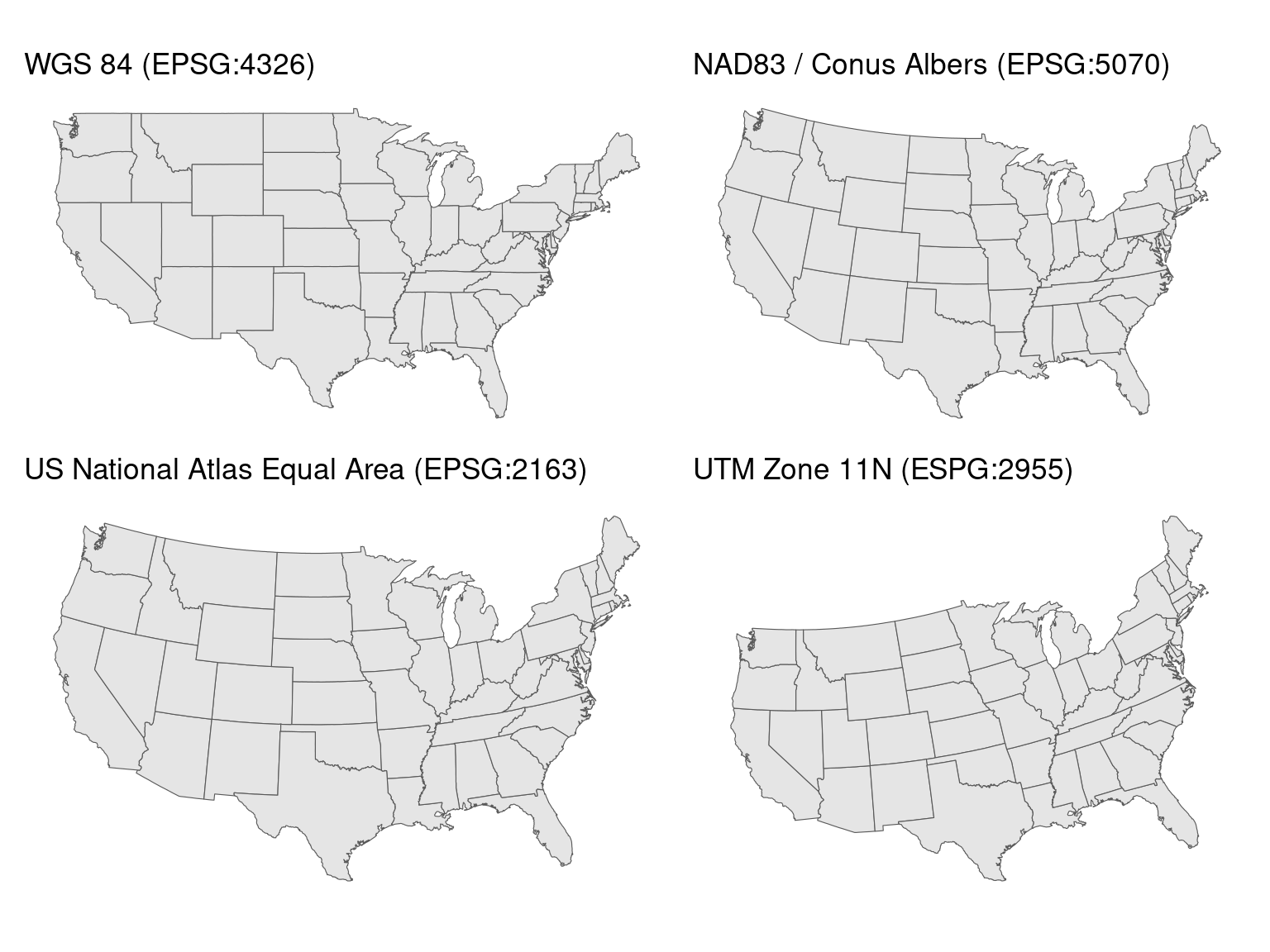
Accurate representations of metadata are important with geospatial data. There are different coordinate reference systems (CRS) which can be used to represent geospatial data, and knowing which one has been used is crucial when combining data from multiple sources.
Saving geospatial data to Arrow format isn’t as simple as taking the data and mapping values to the equivalent Arrow data types. Many geospatial applications have custom data types used to describe the location and shape being represented in the data. These are known as geometries, and can be defined using points, lines, polygons, and other things. These geometries are often stored along with their associated attributes, descriptive information relating to them.
Although these non-standard data types don’t have direct Arrow equivalents, they can be implemented using extension types. Extension types allow you to create custom predefined data types. For example, you could have a location data type for which each value consists of a latitude and longitude float value. That said, there’s a huge range of possibilities for representing geospatial data, and using standardized formats can speed things up when sharing data between platforms.
There are a multitude of different systems for working with geospatial data. Many of the challenges of geospatial data mirror the challenges found working with larger datasets in general: the need for efficient interchange between systems, performance issues on large, complex, or multi-file datasets, and different implementations of overlapping ideas.
GeoParquet was designed to address these issues. GeoParquet provides a standard format for storing geospatial data on disk and can be used with arrow to then represent geospatial data in-memory. The GeoParquet format allows geospatial data to be stored in Parquet files. While it was already possible to store data in Parquet files and have lossless roundtripping between R and Parquet, GeoParquet has the added advantage of being a standardized format for this in the form of a file-level metadata specification.
Working with data in GeoParquet format allows people to take advantage of the same benefits that come with working with any data in Parquet format; the row and column chunk metadata which is an inherent part of Parquet means that filtering on this data can be done without needing to read all data into memory. Parquet’s encoding and compression means that GeoParquet files tend to take up less space on disk than similar formats.
Arrow can read GeoParquet files and perserve the metadata necesary to work with geospatial data efficiently. At the time of writing, there is also a nascent project called GeoArrow designed to make interroperation even easier and more efficient. GeoArrow aims to use the formats and approach of GeoParquet, so should be very similar.
The GeoParquet specification has 2 components: the format of the metadata and then the format of the data itself. There are two levels of metadata:
To make this concrete, we will use geospatial definitions for PUMAs (we will discuss what these are in more detail in Section 7.5.5). This Parquet file has a number of standard columns along with one column, geometry, that includes the geospatial specifications: in this case, polygons and multipolygons, which are the shapes of the PUMAs.
# Read in the puma geoparquet, mark it as such with SF
PUMA <- read_parquet(
  "data/PUMA2013_2022.parquet",
  as_data_frame = FALSE
)The column-level GeoParquet metadata stores 2 different types of information:
GeoParquet specifies 2 different ways of representing geometry data: serialized encoding and native encodings. Native encodings are where this data is stored in Arrow data structures. Serialized encodings are where data is stored in existing geospatial formats. Well-known binary (WKB) data is converted into Arrow Binary and LargeBinary data and Well-known Text (WKT) as Arrow Utf8 or LargeUtf8. This is part of the GeoParquet specification to ensure that this metadata can be preserved without needing to fully convert to the native encoding; however, it can be slower to work with.
Native encoding allows people to full take advantage of working with Arrow data types and capabilities. It provides concrete Arrow data structure to store geometry data in. For example, co-ordinates are stored in one of two Arrow structures. The “separated” approach saves coordinate values in separate Arrow Arrays; one for x values, and one for y values. The “interleaved” approach saves co-ordinate values in a FixedSizeList, and allows x and y values to be stored in an alternating pattern. Other types of geometries are stored in Arrow Arrays or nested ListArrays with a given structure.
For our example, most of the columns are standard types we’ve seen already. But the geometry column is the type binary and specifically the WKB type. Though this looks complicated, it’s very similar to other types: the column is an array of values, effectively a vector in R. The difference is that instead of containing data that are one string per row (that is: UTF8 encoded bytes), this data is one chunk of binary data per row. This binary data is WKB data, which packages like sf can understand.
schema(PUMA)Schema
location: string
STATEFIP: string
YEAR: int32
PUMA: string
GEOID: string
NAMELSAD: string
MTFCC: string
FUNCSTAT: string
ALAND: double
AWATER: double
INTPTLAT: string
INTPTLON: string
geometry: binary
See $metadata for additional Schema metadataThere is also metadata about this column. The most important thing that we care about here is the CRS.
schema(PUMA)$metadata$geo[1] "{\"primary_column\": \"geometry\", \"columns\": {\"geometry\": {\"encoding\": \"WKB\", \"crs\": {\"$schema\": \"https://proj.org/schemas/v0.7/projjson.schema.json\", \"type\": \"GeographicCRS\", \"name\": \"NAD83\", \"datum\": {\"type\": \"GeodeticReferenceFrame\", \"name\": \"North American Datum 1983\", \"ellipsoid\": {\"name\": \"GRS 1980\", \"semi_major_axis\": 6378137, \"inverse_flattening\": 298.257222101}}, \"coordinate_system\": {\"subtype\": \"ellipsoidal\", \"axis\": [{\"name\": \"Geodetic latitude\", \"abbreviation\": \"Lat\", \"direction\": \"north\", \"unit\": \"degree\"}, {\"name\": \"Geodetic longitude\", \"abbreviation\": \"Lon\", \"direction\": \"east\", \"unit\": \"degree\"}]}, \"scope\": \"Geodesy.\", \"area\": \"North America - onshore and offshore: Canada - Alberta; British Columbia; Manitoba; New Brunswick; Newfoundland and Labrador; Northwest Territories; Nova Scotia; Nunavut; Ontario; Prince Edward Island; Quebec; Saskatchewan; Yukon. Puerto Rico. United States (USA) - Alabama; Alaska; Arizona; Arkansas; California; Colorado; Connecticut; Delaware; Florida; Georgia; Hawaii; Idaho; Illinois; Indiana; Iowa; Kansas; Kentucky; Louisiana; Maine; Maryland; Massachusetts; Michigan; Minnesota; Mississippi; Missouri; Montana; Nebraska; Nevada; New Hampshire; New Jersey; New Mexico; New York; North Carolina; North Dakota; Ohio; Oklahoma; Oregon; Pennsylvania; Rhode Island; South Carolina; South Dakota; Tennessee; Texas; Utah; Vermont; Virginia; Washington; West Virginia; Wisconsin; Wyoming. US Virgin Islands. British Virgin Islands.\", \"bbox\": {\"south_latitude\": 14.92, \"west_longitude\": 167.65, \"north_latitude\": 86.45, \"east_longitude\": -40.73}, \"id\": {\"authority\": \"EPSG\", \"code\": 4269}}, \"geometry_types\": [\"MultiPolygon\", \"Polygon\"], \"bbox\": [-179.231086, 13.234188999999999, 179.859681, 71.439786]}}, \"version\": \"1.0.0\", \"creator\": {\"library\": \"geopandas\", \"version\": \"0.14.3\"}}"This is a projjson encoding of the CRS for the geometry column. This encoding is text, which is actually JSON.
jsonlite::fromJSON(schema(PUMA)$metadata$geo)$primary_column
[1] "geometry"
$columns
$columns$geometry
$columns$geometry$encoding
[1] "WKB"
$columns$geometry$crs
$columns$geometry$crs$`$schema`
[1] "https://proj.org/schemas/v0.7/projjson.schema.json"
$columns$geometry$crs$type
[1] "GeographicCRS"
$columns$geometry$crs$name
[1] "NAD83"
$columns$geometry$crs$datum
$columns$geometry$crs$datum$type
[1] "GeodeticReferenceFrame"
$columns$geometry$crs$datum$name
[1] "North American Datum 1983"
$columns$geometry$crs$datum$ellipsoid
$columns$geometry$crs$datum$ellipsoid$name
[1] "GRS 1980"
$columns$geometry$crs$datum$ellipsoid$semi_major_axis
[1] 6378137
$columns$geometry$crs$datum$ellipsoid$inverse_flattening
[1] 298.2572
$columns$geometry$crs$coordinate_system
$columns$geometry$crs$coordinate_system$subtype
[1] "ellipsoidal"
$columns$geometry$crs$coordinate_system$axis
name abbreviation direction unit
1 Geodetic latitude Lat north degree
2 Geodetic longitude Lon east degree
$columns$geometry$crs$scope
[1] "Geodesy."
$columns$geometry$crs$area
[1] "North America - onshore and offshore: Canada - Alberta; British Columbia; Manitoba; New Brunswick; Newfoundland and Labrador; Northwest Territories; Nova Scotia; Nunavut; Ontario; Prince Edward Island; Quebec; Saskatchewan; Yukon. Puerto Rico. United States (USA) - Alabama; Alaska; Arizona; Arkansas; California; Colorado; Connecticut; Delaware; Florida; Georgia; Hawaii; Idaho; Illinois; Indiana; Iowa; Kansas; Kentucky; Louisiana; Maine; Maryland; Massachusetts; Michigan; Minnesota; Mississippi; Missouri; Montana; Nebraska; Nevada; New Hampshire; New Jersey; New Mexico; New York; North Carolina; North Dakota; Ohio; Oklahoma; Oregon; Pennsylvania; Rhode Island; South Carolina; South Dakota; Tennessee; Texas; Utah; Vermont; Virginia; Washington; West Virginia; Wisconsin; Wyoming. US Virgin Islands. British Virgin Islands."
$columns$geometry$crs$bbox
$columns$geometry$crs$bbox$south_latitude
[1] 14.92
$columns$geometry$crs$bbox$west_longitude
[1] 167.65
$columns$geometry$crs$bbox$north_latitude
[1] 86.45
$columns$geometry$crs$bbox$east_longitude
[1] -40.73
$columns$geometry$crs$id
$columns$geometry$crs$id$authority
[1] "EPSG"
$columns$geometry$crs$id$code
[1] 4269
$columns$geometry$geometry_types
[1] "MultiPolygon" "Polygon"
$columns$geometry$bbox
[1] -179.23109 13.23419 179.85968 71.43979
$version
[1] "1.0.0"
$creator
$creator$library
[1] "geopandas"
$creator$version
[1] "0.14.3"And from this we can see that the CRS for our PUMAs is NAD83. We will use this later when we plot the data.
We’ve already read in our geospatial data, and have our PUMS dataset to analyze and plot, and now we need to follow a few more steps to make sure that R plotting libraries like ggplot2 can work with this data.
When this book was being written, there were already nascent projects to make this smoother. sfarrow has tools for reading and writing geospatial data using arrow and the r package geoarrow is under development to make it easier to load data that conforms to GeoParquet and GeoArrow standards.
Today, however, we need to do a couple more things before we can work with it further and use sf and ggplot2 to plot this: make sure that our CRS is set correctly and pulling the data into R. To do both of these, we create a helper function. This helper function ensures that we use the CRS we saw the data had above. It also sets the bounding box and center so that the entirety of the United States is laid out correctly.5 Finally, we pull the data into R and set the correct geometry column to use.
correct_projection <- function(PUMA, crs = "NAD83") {
  PUMA_df <- collect(PUMA)
  # set the geometry column, but we also need to manually
  # extract the CRS from the geoparquet metadata
  PUMA_df <- sf::st_sf(PUMA_df, sf_column_name = "geometry",
                       crs = crs)

  # Move the bounding box + center of the projection so that
  # Alaska is plotted together
  proj <- paste(
    "+proj=aea",
    "+lat_1=29.5",
    "+lat_2=45.5",
    "+lat_0=23",
    "+lon_0=-96",
    "+x_0=0",
    "+y_0=0",
    "+ellps=GRS80",
    "+towgs84=0,0,0,0,0,0,0",
    "+units=m +no_defs"
  )
  PUMA_df$geometry <- st_transform(PUMA_df$geometry, crs = proj)

  PUMA_df
}Putting this all together, let’s try making a plot6 showing different languages spoken throughout the United States. The analysis we will build up is the percentage of speakers for languages spoken in the US. We will then plot this data, subsetting to a few interesting languages depending on what region we are plotting. In the PUMS dataset, the smallest geographic area is called a PUMA (Public Use Microdata Areas).7 These PUMAs are designed to have approximately 100,000 people in them, and must be within a single state.
As always, we start with our PUMS dataset. We build up a dplyr query to clean some data inconsistencies, such as varying capitalization, then group by language and PUMA by state and year, and calculate how many speakers of each language there are in each PUMA. We can see that this returns a data frame with one row per PUMA and language, with the number of speakers and the proportion of speakers whose primary language is not English compared to the overall population.
pums_person <- open_dataset("./data/person")

puma_by_langauge <- pums_person |>
  filter(year == 2018) |>
  mutate(
    language = tolower(LANP),
    language = case_when(
      is.na(language) ~ "english",
      TRUE ~ language
    )
  ) |>
  filter(language != "english") |>
  group_by(location, PUMA, year, language) |>
  summarize(
    n_people = sum(PWGTP)
  ) |>
  group_by(location, PUMA, year) |>
  mutate(
    prop_speaker = n_people / sum(n_people),
  ) |>
  ungroup()

puma_by_langauge |>
  head() |>
  collect()
And then we can take that data, join it to our arrow table of PUMAs and plot it using ggplot2. There is one other cleaning step we need, though, and we’ve factored it out into a fill_pumas() function. The function is a wrapper around some dplyr joins to make it so that each PUMA has one row for each language. Because many languages are not spoken at all in many PUMAs, we need to do this so that the plots still show those PUMAs as 0, not NA.
fill_pumas <- function(query) {
  # unique combination of every state + puma + year
  unique_pumas <- query |>
    distinct(location, PUMA, year) |>
    # add `key` as a constant so we can join with `unique_languages`
    mutate(key = 1)

  # all of the languages
  unique_languages <- query |>
    distinct(language) |>
    mutate(key = 1)

  # crossed together
  pumas_languages <- unique_pumas |>
    full_join(unique_languages) |>
    select(-key)

  # return the original query with all of the
  # unique combinations, when those values are
  # NA, make them 0
  query |>
    right_join(pumas_languages) |>
    mutate(
      n_people = coalesce(n_people, 0),
      prop_speaker = coalesce(prop_speaker, 0)
    )
}
Note that, as we discussed in Section 3.5, none of the steps in fill_pumas() calls collect() or compute(): they are all adding steps to the query without evaluating it.
Now we’re ready to plot.
puma_by_langauge |>
  filter(language %in% c("german", "spanish", "french", "navajo")) |>
  fill_pumas() |>
  inner_join(
    PUMA,
    by = c("year" = "YEAR", "location" = "location", "PUMA" = "PUMA")
  ) |>
  correct_projection() |>
  ggplot() +
  geom_sf(aes(geometry = geometry, fill = prop_speaker),
          lwd = 0) +
  coord_sf(crs = "+proj=laea +lon_0=-98 +lat_0=39.5") +
  facet_wrap(vars(language), ncol = 2) +
  scale_fill_distiller(type = "seq", direction = 1,
                       palette = "Greys",
                       name = "proportion of speakers") +
  theme_minimal() +
  theme(legend.position = "bottom") +
  labs(
    title = "Proportion of non-English speakers by language",
    subtitle = "across the US by PUMA"
  )
We can clearly see some patterns of migration: French is spoken in parts of northern Maine and Louisiana; German is spoken in the midwest, especially in the upper midwest and intermountain west.
That plotting code might look intimidating at first, but most of it is to add theming and to get the projection on the globe. Breaking this down chunk by chunk:
ggplot() +The standard start to ggplot2.
  geom_sf(
    aes(geometry = geometry, fill = prop_speaker),
    lwd = 0
  ) +
Set the geom to be a map, with the color proportion of speaker. Also set the line width of the outlines of each PUMA to be none.
coord_sf(crs = "+proj=laea +lon_0=-98 +lat_0=39.5") +This shifts the projection slightly to be as if it were on a globe.
facet_wrap(vars(language), ncol = 2) +Making small multiples for each language
  scale_fill_distiller(type = "seq", direction = 1,
    palette = "Greys", name = "proportion of speakers") +
  theme_minimal() +
  theme(legend.position = "bottom") +
  labs(
    title = "Proportion of non-English speakers by language",
    subtitle = "across the US by PUMA"
  )
And finally, the theme, labels, title, and color scale.
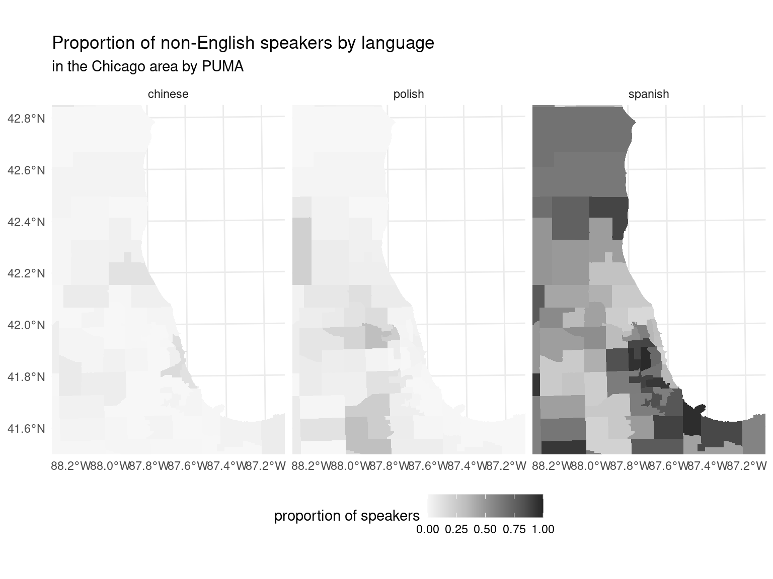
With geospatial plotting, the more detailed a plot is, the larger amount of data needs to be processed to make the plot. At that scale, it can be hard to see just how detailed this map ends up being. Not only are the coastlines detailed, but the PUMAs themselves are quite small with their own unique borders. We can zoom in on the area around Chicago to see just how detailed these get. We’ve selected slightly different languages for each area to highlight unique distributions, like the relatively large number of Polish speakers in the Chicago metro area.
puma_by_langauge |>
  filter(language %in% c("chinese", "spanish", "polish")) |>
  fill_pumas() |>
  inner_join(PUMA, by = c("year" = "YEAR",
                          "location" = "location",
                          "PUMA" = "PUMA")) |>
  correct_projection() |>
  ggplot() +
  geom_sf(aes(geometry = geometry, fill = prop_speaker),
          lwd = 0) +
  coord_sf(
    xlim = c(000000, 100000),
    ylim = c(000000, 150000),
    crs = "+proj=laea +lon_0=-88.3 +lat_0=41.5",
    expand = FALSE
  ) +
  facet_wrap(vars(language), ncol = 3) +
  scale_fill_distiller(type = "seq", direction = 1,
                       palette = "Greys",
                       name = "proportion of speakers") +
  theme_minimal() +
  theme(legend.position = "bottom") +
  labs(
    title = "Proportion of non-English speakers by language",
    subtitle = "in the Chicago area by PUMA"
  )
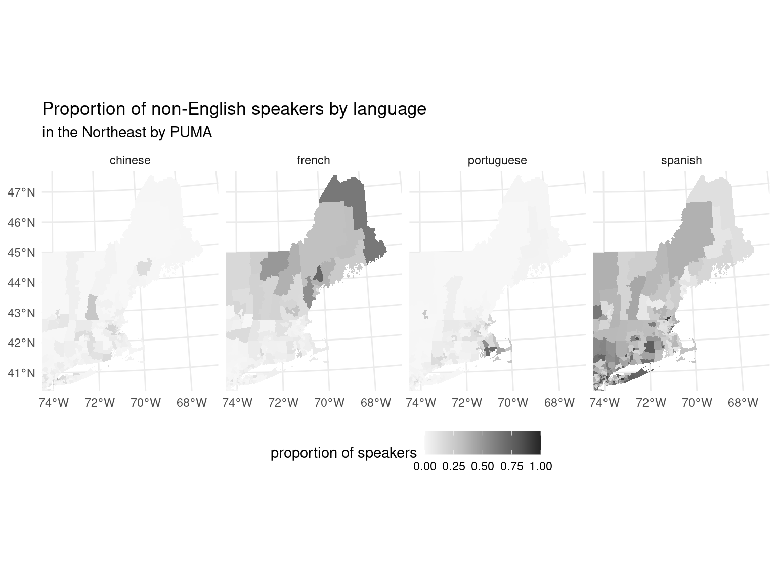
Or the Northeast, where there are a relatively large proportion of Portugese speakers in Massachusetts, and French speakers in Northern Maine.
puma_by_langauge |>
  filter(language %in% c("chinese", "spanish", "french",
                         "portuguese")) |>
  fill_pumas() |>
  inner_join(PUMA, by = c("year" = "YEAR",
                          "location" = "location",
                          "PUMA" = "PUMA")) |>
  correct_projection() |>
  ggplot() +
  geom_sf(aes(geometry = geometry, fill = prop_speaker),
          lwd = 0) +
  coord_sf(
    xlim = c(000000, 650000),
    ylim = c(000000, 810000),
    crs = "+proj=laea +lon_0=-74.5 +lat_0=40.4",
    expand = FALSE
  ) +
  facet_wrap(vars(language), ncol = 4) +
  scale_fill_distiller(type = "seq", direction = 1,
                       palette = "Greys", name =
                         "proportion of speakers") +
  theme_minimal() +
  theme(legend.position = "bottom") +
  labs(
    title = "Proportion of non-English speakers by language",
    subtitle = "in the Northeast"
  )
This chapter explored advanced topics for working with the arrow R package. We began talking about user-defined functions (UDFs), explaining how to create and utilize them to handle functions not natively supported by Arrow. We also looked at the interoperability between Arrow and DuckDB, showing how to use DuckDB for tasks not natively supported in Arrow. Finally, we took a look at extending arrow, with a focus on geospatial data, introducing the concept of GeoParquet for on-disk geospatial data representation that can quickly and easily be turned into an in-memory representation.
Acero doesn’t have a logical query optimizer, but as we have seen, it does support optimizations like “predicate pushdown” - filtering the data where it is stored rather than in memory, which is what makes filtering on partitioned datasets fast. To take advantage of these optimizations, there is code in the R package that reorders queries before passing it to Acero for most common workflows.↩︎
Overflow is when a numeric value is larger than the type can support. For example, unsigned 8 bit integers can represent numbers 0-255. So if we add 250 + 10 we would have a value that is 260, which is not able to be represented with 8 bits. The checked variants of arithmetic calculations will raise an error in this case, which is almost always what we want in these circumstances.↩︎
They better be very close since this is the same data the linear regression was fit with!↩︎
Without this, some of the Aleutian islands which are to the west of the 180th meridian will be plotted to the east of the rest of the United States.↩︎
This type of plot is called a choropleth where a geographic representation is colored or shaded to show different values in different areas.↩︎
There is also a more detailed description of PUMAs in Kyle Walker’s Analyzing US Census Data: Methods, Maps, and Models in R ↩︎